


One of the amazing things about Microsoft Fabric is the number of options you have for moving data. For example, you can use Dataflow Gen2, Pipelines, Notebooks, or any combination of the three.
However, with all the options available, it can also make deciding which pattern to use a bit like reading the menu at The Cheesecake Factory. Hopefully, this article will help shed some light on the pros and cons of each approach while also showing you how they impact the elephant in the room: Capacity Units (CUs).
Before we dive in, we need to understand a few things. Let's start with the most important topic: understanding how your capacity consumption is measured.
* Disclosure: Due to a correction of a record duplication issue, some modifications have been made to the original publication of this article. For transparency, I will identify the impact throughout the article with comments and (bold) identifers.
Brief Capacity Overview
Premium Capacity has been around for a few years as part of the Power BI stack. However, until the release of Fabric, you only had to worry about how Power BI impacts your capacity. With Fabric, "all" experiences have been standardized to use the same serverless compute, meaning pipelines, notebooks, SQL endpoints, and so on, which all consume compute from your available capacity pool. Because of this, it's more important than ever to truly understand the cost of each workload.
Like Power BI Premium, Fabric capacities have many SKUs, each giving you a specified amount of compute to work with.
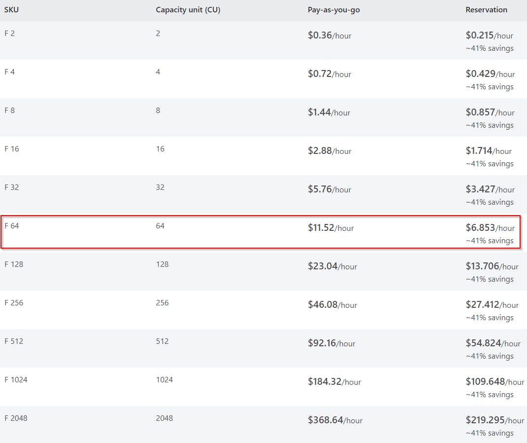
There's an additional SKU that isn't listed, FT1 or Fabric Trial Capacity. The FT1 is equivalent to the F64 SKU, which is also equivalent to the existing Power BI P1 SKU.
All tests performed in this article were done so using an FT1.
Capacity Metrics: First Look
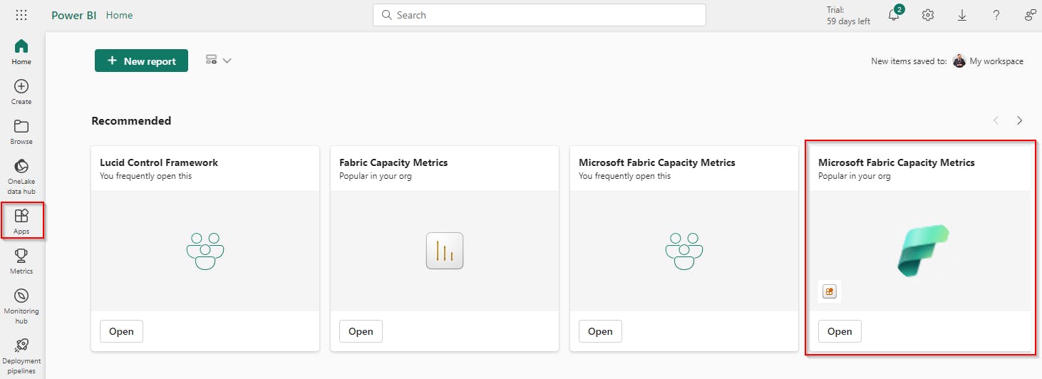
To begin understanding your capacity consumption, the Microsoft team has created a Fabric Capacity Metrics app that can be deployed from the Power BI app collection. Go to the Apps section of your left-side navigation, click "Get apps" in the top right, and search Fabric.
Once you have the app installed, you'll need to authenticate and make a few selections regarding the configuration of the timezone and such; it's quite straightforward, though.
Alas, you're ready to see the magic! Well, it's not quite magic, but it's a starting point. The app has a few challenges, as you'll soon encounter, but perhaps the biggest challenge is having only a rolling 14 days available. This makes historical analysis quite challenging. There are ways around this which I'll cover in a later article, for now let's stay on topic.
Upon taking your first look at the metrics, your first thought might be, "What the heck am I looking at?" With all analysis, unless you understand the numbers, they're just numbers. It's a movie without a plot. They exist, but what do they mean? What story are they telling?
Capacity Unit: The Numbers
For our analysis, we will hone in on a specific data point: CU(s).
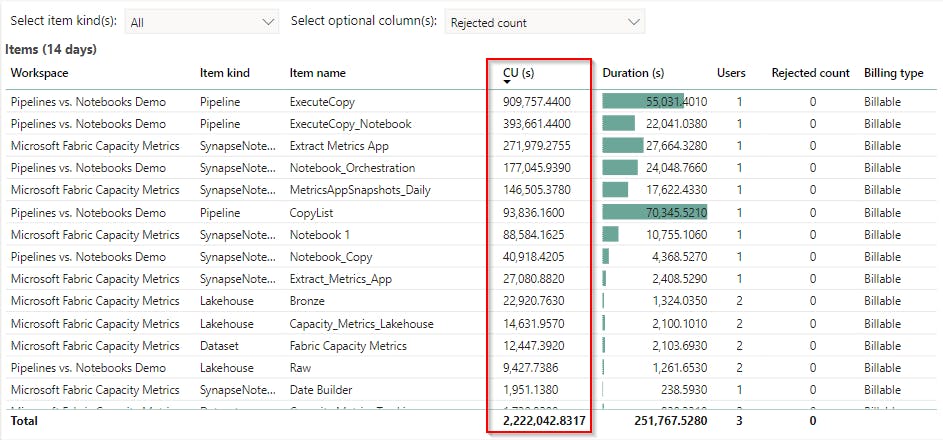
These look like big numbers. These activities must be super expensive, right? Like the old Transformers theme song, there's "more than meets the eye."
To understand the true cost of an activity, we have to do some math. Referring to the chart in the previous section, we're using the equivalent of an F64, which means we have 64 Capacity Units at our disposal. To translate that, we must first understand what a Capacity Unit is. Let's break it down.
First and foremost, a Capacity Unit is not the same as a CU(s). A Capacity Unit is a measurement based on hours, as indicated here:


CU(s) is a measurement of seconds, which can be misleading. I initially thought the Duration was somehow used in the conversion, but this is not true. The conversion of Capacity Unit to CU(s) is as follows:
1 Capacity Unit (hour) = 60 seconds * 60 minutes = 3,600 (seconds per hour)
For our F64 (FT1) with 64 Capacity Units:
64 Capacity Unit (hour) = 3,600 CU(s) * 64 = 230,000 CU(s) per hour
To translate this to cost, I'll use the first row from the capacity metrics app screenshot above with a CU(s) consumption of 909,747.44.
With our understanding of the conversion between CU(s) and Capacity Units, we can convert CU(s) to cost:
Capacity Units = 909,747.44 CU(s) / 3,600 = 252.707622222
PayGo Cost per Capacity Unit = $11.52 / 64 = $0.18
PayGo Cost (USD) = 252.71 * $0.18 = ~$45.49
Reservation Cost per Capacity Unit = $6.853 / 64 = $0.107078125
Reservation Cost (USD) = ~$27.06
If you really wanted to break it down further to determine the cost per CU(s):
PayGo Cost per Capacity Unit = $11.52 / 64 = $0.18
PayGo Cost per CU(s) = $0.18 / 3,600 = $0.00005
Reservation Cost per Capacity Unit = $6.853 / 64 = ~$0.107078125
Reservation Cost per CU(s) = $0.107078125 / 3,600 = ~$0.000029744
Now that you understand the meaning behind the numbers let's dig into the real purpose of this article.
For the remainder of the article, any cost-related metrics will be calculated using the Reservation rate.
All Experiences Were Not Created Equal
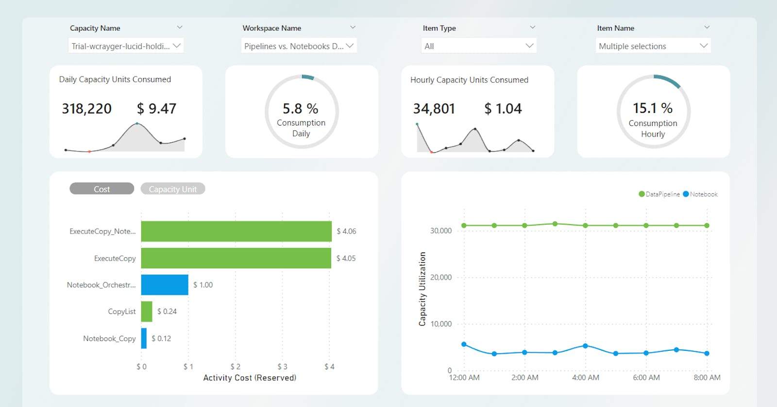
To make this a bit easier to digest, I've created a monitoring report to help me tell the story.
Welcome to the Lucid capacity monitoring report!
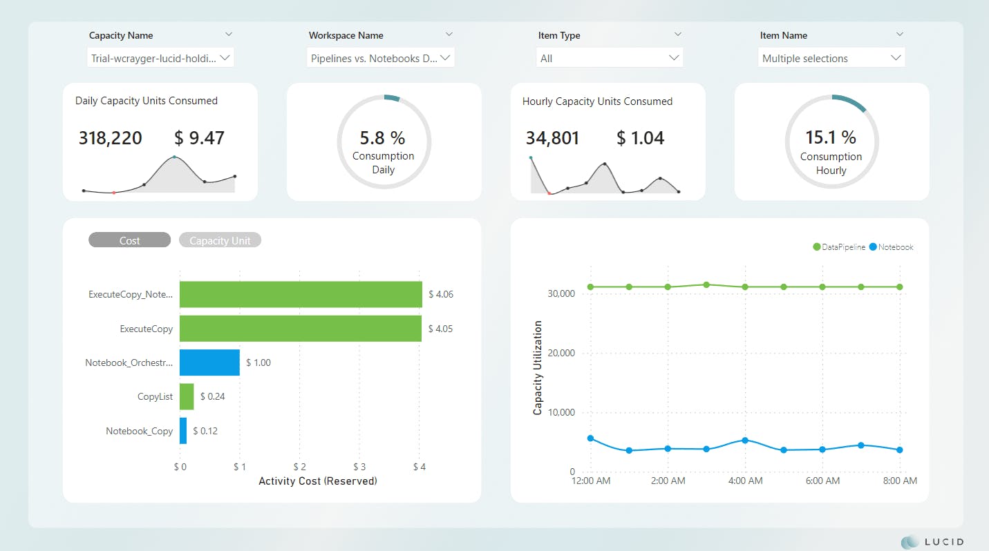
*Image updated
The custom monitoring report uses a combination of data elements from the Fabric tenant as well as data points captured directly from the Fabric Capacity Metrics app. The backend of this report is a Fabric Lakehouse that's being populated by a Spark notebook in scheduled intervals.
The notebook has been written to perform the following operations:
Refresh the Fabric Capacity Metrics semantic model
Capture data about the Fabric tenant, such as workspace, capacity, and item details, into a series of stage tables
Create a calendar stage table
Perform a dynamic UPSERT from the stage tables to a set of dimensional tables
The Lucid monitoring report is then connected to a semantic model of the Lakehouse via Direct Lake mode.
Setting The Stage
For our comparisons, we will focus on different processing patterns using Pipelines and Notebooks. The three patterns I'll be reviewing are a traditional pipeline pattern using nested pipelines with a ForEach loop, using a notebook to generate the list that is passed to a single pipeline via API, and using a notebook to generate the list as well as "copy" directly from the source.
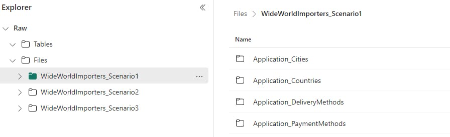
Each scenario follows the same structure, reading data from the source and writing a parquet file to a designated folder in a Lakehouse.
All tests were scheduled to run hourly and performed at staggered intervals to minimize the potential of a noisy neighbor impacting the test.
I used the WideWorldImporters OLAP database hosted in an Azure SQL database for sample data. To simulate real-world examples, I have a daily pipeline to execute a stored procedure that populates fresh data.
Sample:
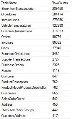
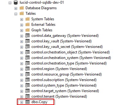
Additionally, each pattern uses a basic metadata-driven approach consisting of a single Azure SQL database containing a few control tables. There are a total of 44 tables that are processed as part of my testing.
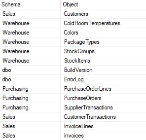
dbo.Copy sample:
My testing aimed to understand the efficiency and consumption of each processing pattern with respect to Fabric workloads.
Traditional Parent / Child Pipeline Pattern
A simple and efficient pattern to dynamically process data using pipelines is to use a parent/child relationship. In this pattern, a parent pipeline typically generates a list of items to process before passing the items in the list to a ForEach loop.
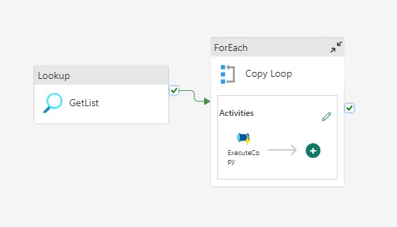
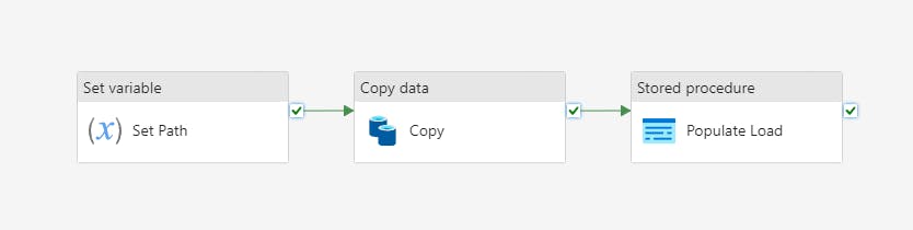
Inside the ForEach loop is usually an activity to execute another pipeline, the child. In this example, the child pipeline sets the path where the parquet file will be written, performs the copy, and logs the path for later retrieval.
Scenario 1 Results
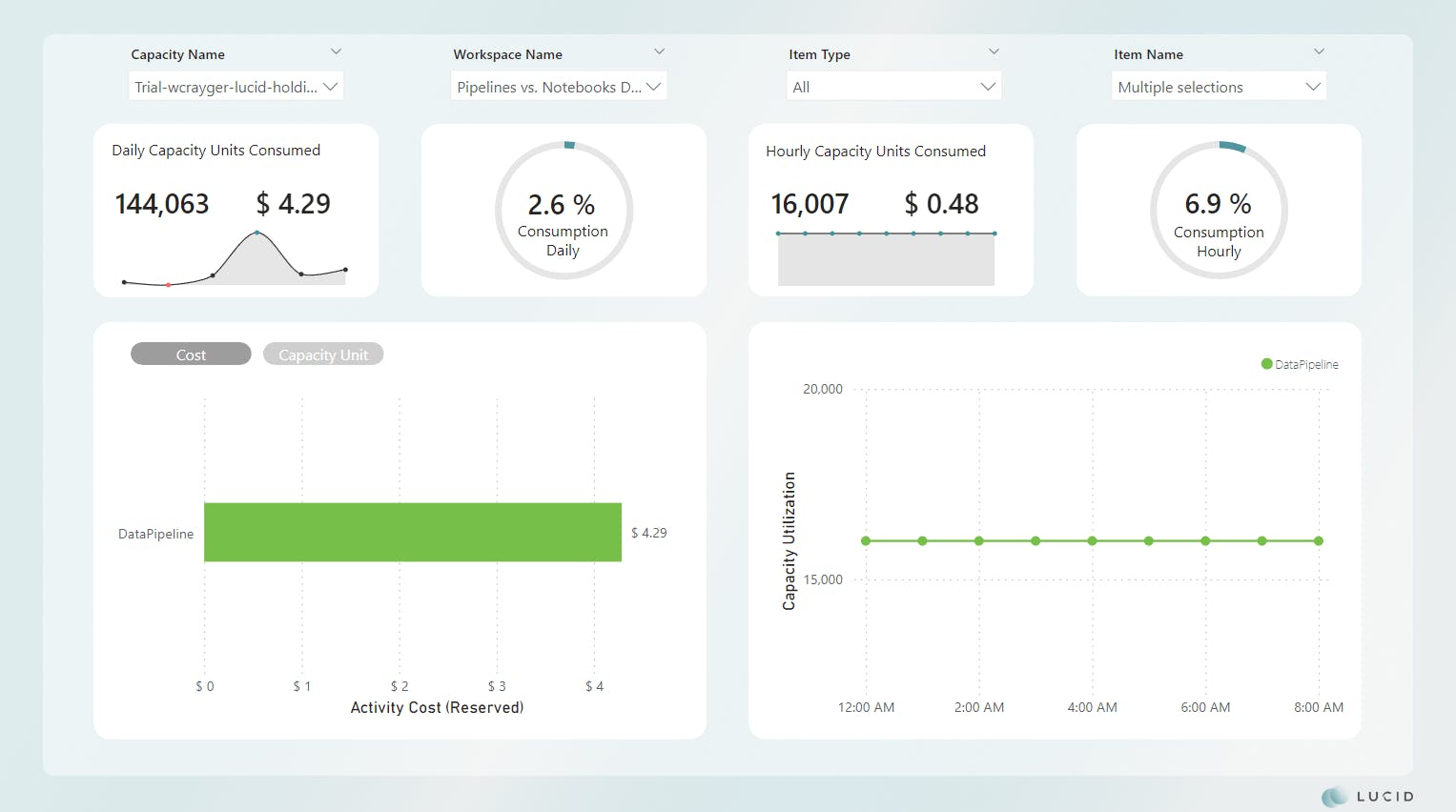
*Image updated
The test for this pattern was quite interesting. Repeating values. Why are there repeating values? I thought maybe I had a bad measure or was missing a relationship. I went back to my Lakehouse to check the data. Interestingly, the capacity units consumed remain static, but the activity duration and other metrics fluctuate.
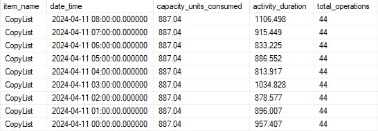
*Image updated
Looking at the child pipeline, we see the same pattern.
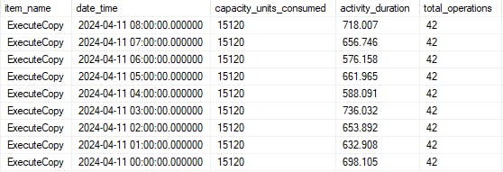
*Image updated
This looks like the "smoothing" is kicking in and spreading the total consumption of the runs out. That said, I'm not 100% sure and would like to dig in more to confirm my suspicion.
For now, let's continue and focus on the total consumption for all runs in the day. As we can see from our report, this pattern cost us $4.29 for the day and consumed 2.6% of the total available daily compute.
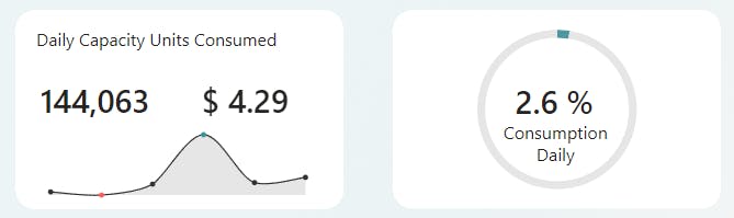
*Image updated
Notebook Orchestration with Pipeline Copy
The next scenario I wanted to test combines the use of both a pipeline and a notebook. In this pattern, we use a notebook to replace the parent pipeline from Scenario 1.
There are several reasons as to why you may want to do this. Pipelines are efficient at copying data but can often be too rigid regarding lookups or other configuration requirements, especially when working with metadata frameworks. Because of this, developers will begin to include multiple layers of nested pipelines, which can become quite expensive.
By combining the use of a notebook to build the configuration and a pipeline to perform the copy, you have much more flexibility and control over your process.
# Function to be executed in parallel for each row to call API
def call_api_with_payload(row, workspace_id, item_id, job_type, client):
    """
    Orchestration pattern consumption analysis
    Tests performed by Will Crayger of Lucid
    """

    # Extract parameters for payload from the row
    payload = {
        "executionData": {
            "parameters": {
                "schema": row["Schema"],
                "object": row["Object"],
            }
        }
    }

    # Call the Fabric REST API
    try:
        response = client.post(f"/v1/workspaces/{workspace_id}/items/{item_id}/jobs/instances?jobType={job_type}", json=payload)
        if response.status_code == 202:
            pass
        else:
            return response.json()
    except Exception as e:
        # Print error
        print(f"An error occurred while calling API: {e}")
        return None

# Retrieve processing list
process_list_sql = "SELECT * FROM [dbo].[Copy]"
df_process_list = spark.read.format("jdbc").option("url", key_vault_secret).option("query", process_list_sql).load()

# Convert to Pandas DataFrame
df_pandas = df_process_list.toPandas()

# Define parameters for scheduler
workspace_id = fabric.get_workspace_id()
item_id = "<your_item_id>"
job_type = "Pipeline"

# Use ThreadPoolExecutor to call APIs concurrently
with ThreadPoolExecutor(max_workers=min(len(df_pandas), (os.cpu_count() or 1) * 5)) as executor:
    # Submit tasks to the executor
    future_to_row = {executor.submit(call_api_with_payload, row, workspace_id, item_id, job_type, client): index for index, row in df_pandas.iterrows()}
Scenario 2 Results
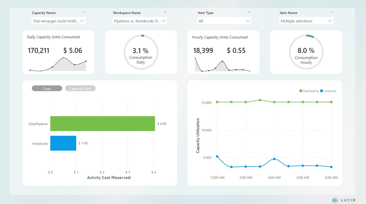
*Image updated
There are currently a few challenges with this approach in Fabric. One challenge is there appears to be a limited set on the API itself that only allows 10 connections. Any more than 10 connections are throttled, queued, and executed when previous connections are closed. I wasn't able to find this in the documentation, though.
Further investigation shows the CU(s) required for the pipeline execution itself are comparable to that of the Scenario 1 ExecuteCopy activity. The decrease in efficiency is attributed to the notebook remaining active during the API throttling.
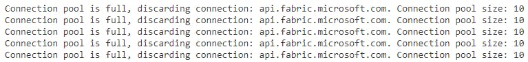
https://learn.microsoft.com/en-us/rest/api/fabric/articles/throttling
Scenario 1:
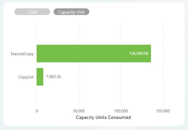
Scenario 2:
This is also visible on the monitoring hub, as only 10 pipeline executions will trigger at once. As you can also see, the Notebook_Orchestration activity remains in an "In Progress" status until all pipelines have been executed, thus increasing consumption.
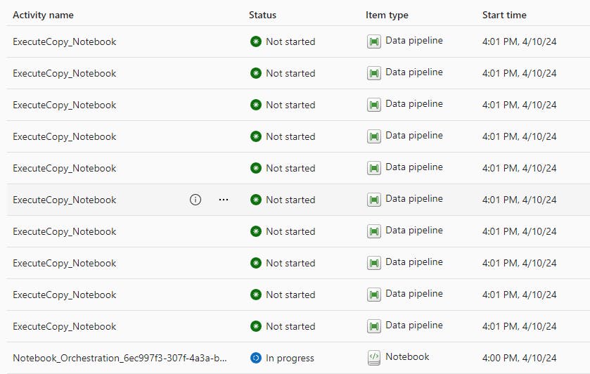
My initial thought was to bypass the Semantic Link API and try a potential workaround, but I soon remembered the next challenge with this approach. There's currently no support for service principal authentication, meaning using another API strategy is a no-go.
Scenario 2 yielded a ~18% decrease in efficiency and cost compared to Scenario 1.
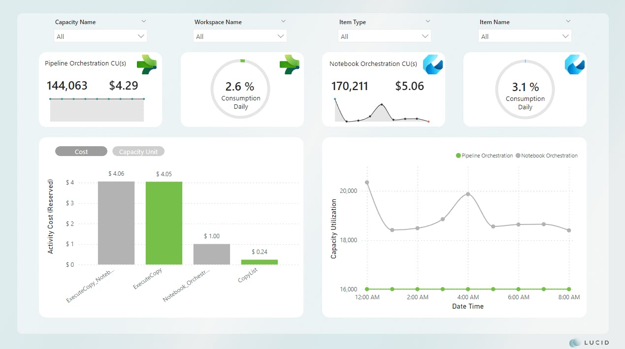
*Image updated
Notebook Orchestration and Copy
The final scenario I tested was using a notebook to orchestrate and copy the data.
For years, we've relied on pipelines, and before pipelines, we used tools like SSIS to create orchestration packages. We've used this pattern for so long that it's become muscle memory. There's a reason for this, though. They're easy to use!
Setting up a pipeline is as simple as clicking through a GUI these days, and with the ability to integrate things like Dataflows Gen2, things will only get easier. However, ease comes with a significant cost.
Spark processing in tools like Fabric and Databricks opens the door to more programmatic ETL/ELT patterns like the one below.
def read_source_data(row):
    """
    Orchestration pattern consumption analysis
    Tests performed by Will Crayger of Lucid
    """
    try:

        # Create dynamic SQL using the row values
        dynamic_sql_query = f"SELECT * FROM [{row['Schema']}].[{row['Object']}]"

        # Read source data to DataFrame and write to Delta
        df_source = spark.read.format("jdbc") \
                    .option("url", source_connection) \
                    .option("query", dynamic_sql_query) \
                    .load()

        # Set staging table name using the row values
        stage_file = f"Files/WideWorldImporters_Scenario3/{row['Schema']}_{row['Object']}"

        # Write to delta
        df_source.write.format("parquet") \
            .mode("overwrite") \
            .save(stage_file)
    except Exception as e:
        print(f"Error processing {row['Schema']}_{row['Object']}: {e}")

# Retrieve processing list and convert to Pandas DataFrame
process_list_sql = "SELECT * FROM [dbo].[Copy]"
df_process_list = spark.read.format("jdbc") \
                    .option("url", control_connection) \
                    .option("query", process_list_sql) \
                    .load()
df_process_list_pandas = df_process_list.toPandas()

# Use ThreadPoolExecutor to execute the function in parallel for each row
max_workers = min(len(df_process_list_pandas), (os.cpu_count() or 1) * 5)
with ThreadPoolExecutor(max_workers=max_workers) as executor:
    # Submit tasks to the executor for each row in the Pandas DataFrame
    futures = [executor.submit(read_source_data, row) for index, row in df_process_list_pandas.iterrows()]
In this example, you'll notice 2 SQL executions, one to retrieve the list of objects to process and the other to execute a SELECT against the source system using a JDBC connection. You'll also notice the use of ThreadPoolExecutor, which allows for parallel execution.
Scenario 3 Results
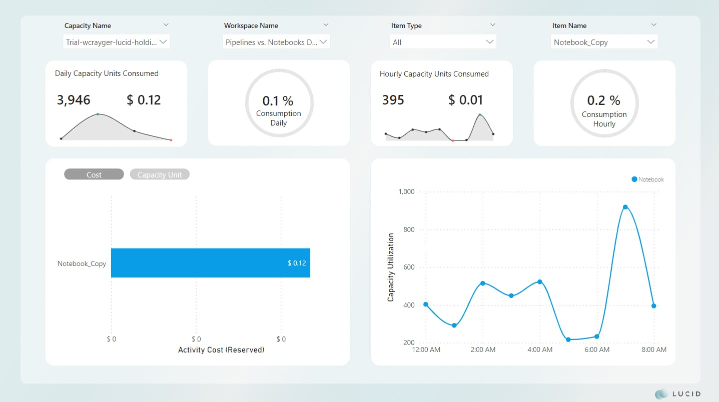
*Scenario 3 was not impacted and remains unchanged
If you're at a loss for words, don't worry; I was right there with you when I saw the results. Absolutely shocking!
Now, this approach isn't without considerations. Traditionally, this scenario can be challenging for on-premise environments or sources behind a firewall of some sort. The Fabric team has rolled out several new features, such as VNET and gateway integration, to alleviate some of these concerns. Another consideration is not all sources will support direct reads using Spark.
Let's look at the comparisons by the numbers.
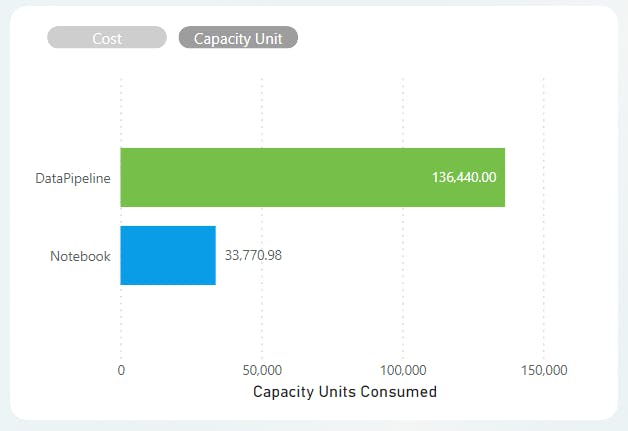
Scenario 2 vs. Scenario 3
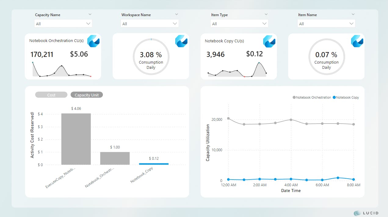
*Image updated
Scenario 1 vs. Scenario 3
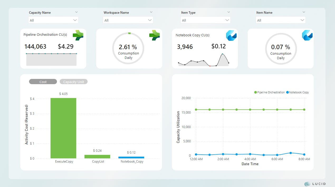
*Image updated
Comparisons show an improvement of ~98% for cost and CU(s) consumption across the board.
Final Thoughts
As the numbers show, traditional metadata patterns, while easy, can also be incredibly costly. Every data team should review and potentially redesign their frameworks to address these inefficiencies.
At Lucid, I've begun following a Spark-first approach and will only use Pipelines when required. I've also developed a framework to quickly deploy and integrate within my client environments, allowing them to focus on decision-making and giving them back their most valuable asset, time.
If you'd like to learn more about how Lucid can support your team, let's connect on LinkedIn and schedule an intro call.